
Development and release log
May 18 2011: 1.1.1
Resolved two issues:
1) on some platforms, access to the runtime arguments (the name of the xml file to run)
was giving erroneous strings padded with junk rather than blanks. Trimming these strings therefore gave
spurious names for the files in which the results were saved.
2) An initialization problem in the core calculations for empty synapse populations caused an array overwrite and correspondfing nasty problems. It was assuming synapses[n_synapses] would always exist, wherease it doesn't if n_synapses=0 (array indexes running from 1 to n_synapses).
January 22 2010: 1.09 Increased the workspace for random numbers to support larger populations of stochastic channels. There should now be better error reporting too if the same problem occurs in future.
January 26 2010: 1.08 You can now have more than one DensityAdjustment element, so, for example, different channel types can be used on different regions of the cell. The DensityAdjustment elements are applied in sequence and each only affects the region in which both channel types are present.
January 22 2010: 1.07 Support for explicit sequences of synaptic events. Previously the ability to read an event sequence from an external file (EventSequence) was documented but not implemented. Now it is read and processed in Java and supported by the fortran core.
June 10 2009: 1.05 removed unnecessary warning about not finding synapse populations: it wasn't finding them, but it also didn't need to as they were dereferenced independently after parsing the xml.
May 11 2009: channel initialization. The channels were being initialized by an method for computing eigenvectors that was formally equivalent to letting the channels relax for 2^16 (about a million) timesteps. It turns out that this isn't always enough for some models (eg arising from a dodgy temperature scaling that gives extremely slow transition rates - the biological relevance of such models could be questionable) particularly if using very small timesteps. Now it computes a separate set of transition matrices at the initial potential and uses them. The process is independent of the timestep and equivalent to letting the channels relax at the starting potential for 1000 seconds.
April 21 2009: variable discretization. There is not the option to set different values for the discretization parameter across the structure as in:
<StructureDiscretization baseElementSize="45.um">
       <LocalRefinement from="752" elementSize="5um" />
    </StructureDiscretization>
January 12 2009: various usability enhancements There is a new option separteFilesExtension for recording configurations so that you can change hte default file name extension from '.txt' when the output is split into one file per column. The recordClamps flag is now an attribute of the recording configuration, not of the main mode. Removed a warning about not recognizing the smart recorders (this was just for the label on the default image of recording locations). Extended the random number work array to avoid overruns.
January 12 2009: voltage clamp behavior. There was an instability in the treatment of voltage clamps on multi-compartment structures in earlier version. This has been fixed by keeping proper track of all clamped compartments and segrerating the solution matrix accordingly.
December 9 2008: NeuroConstruct compatibility: various bug fixes and modifications to facilitate integration with NeuroConstruct.
- New units kohm and kohm_cm
- Fixed problem parsing numbers in scientific notation with negative exponents (like "1.2e-8")
- New optional attribute on the main PSICSRun block: outputFolder. If specified this sends output to the specified folder rather than the default which is to create a folder where the model definition is using the root of the main mode file as the folder name.
- New label attribute on clamps and recorders for recording configurations. These are used for the column headings in the resulting text file.
- New separateFiles flag on a recording configuration to cause the separate columns of the output file to be put in separate files. The file names are as for the multi-column file with "-" and the column heading appended.
- The View elements for the default display no longer need limits (xmin, xmax, ymin, ymax). If these are not there, then the range is chosen to display all the data.
With these changes, a recording file can look like:
<Access id="recording" separateFiles="true">
	<CurrentClamp label="start" at="p0" lineColor="red" hold="0.1nA" />
	<VoltageRecorder label="end" at="p1" lineColor="blue" />
</Access>
For the plot generation, a minimal ViewConfig now looks like:
<ViewConfig>
	<LineGraph width="500" height="400">
		<XAxis label="time / ms" />
		<YAxis label="potential / mV" />
		<LineSet file="psics-out.txt" color="red" />
		<View id="whole" />
	</LineGraph>
</ViewConfig>
October 21 2008: New RunSet option: merge to merge the separate output files into a single file. The first column is discarded from all but the first file and they are joined as successive columns of a table. There is not much error checking as yet, so only use this if you know the files can be meaningfully merged. In particular, if the parameter being varied in the RunSet is the timestep or the runtime, then it is probably not useful to set the merge flag.
October 21 2008: there is a new flag on the main configuration file, recordClamps that sets whether voltage and current clamps should also be treated as recorders and produce columns in the output file. The default is 'true', but it can be useful to set it to 'false' if there are a lot of clamps and the resulting files are large. In this case, recorders should be attached to the sites you want to record from. N.B. There is also a record flag on individual clamps but the core currently ignores it.
May 30 2008: removed restriction on the number of recording sites (it was 100), and added a "column" attribute to TimeSeries elements so that a single master file can contain inputs for many sites. Several TimeSeries elements can refer to the same file and specify which column to use (column numbers begin at 1. Column "0" contains the times).
April 16 2008: Improved treatment of orientation synchronization between projected and java3D views.
Forum running on psics.org for announcements, questions and suggestions.
April 15 2008: Index on the formats page for all elements and attributes and a search box at the top right. The search results should improve when access restrictions are removed, and the page titles are now more informative but it will take a while for these to appear in Google.
April 14 2008: Log/log option and example for power spectrum plots. Improved handling of Neuron morphology exports (supporting model view version 5.9) without any manual editing, even if some of the XML is invalid. New documentation in cell properties reference section for density adjustments.
April 7 2008 - Raster images: new Raster option within ViewConfig to generate a spike raster plot from multiple runs. See the "raster" model for an example of usage and the corresponding output.
April 7 2008: additional output format from FPSICS for multiple runs. When multiple runs are specified for a model, the runs are performed one after another with the data accumulating in a binary output file. Normally, the results are transposed when the equivalent text file is produced so that there is one column per run. This process is inappropriate for very large numbers of runs (more than a thousand or so) because of memory requirements and limited support for ascii tables with such large numbers of columns. For these cases an alternative text format is used that maintains the sequential storage of separate runs. This makes it slightly harder to read the whole thing at once (which is unlikely to be useful in any case) but makes sequential processing much simpler.
Morphology display on output. There is now a view of the morphology in results files with stimulation and recording sites labeled.
X3D output. Icing now supports and "export" function to write the morphology and channels as an X3D file (the successor to VRML). This can be read by a range of independent 3D viewers and may be useful for generating high-resolution images or for 3D visualization without using Java 3D.
March 30 2008: Version 0.8.2 - resolved two problems with external morphology sources. First, on saving a morphology in PSICS from at from Icing, the newly written object was being reread and then replaced by a dummy object. This was just redundant code from before the importer worked, and has now been removed. Second, there were still problems with root points on the discretization of some morphologies. The case where the root of the structure (the soma) is expressed just as a wider part of a continuous section needs special treatment. Looking at the center point after discretization, most cases with two neighbors form a monotonic sequence from one neighbor to the center point to the other neighbor. But this doesn't hold for the root point, which needs the order of internal points to one of the neighbors to be reversed.
March 05 2008: Resolved a problem with HH sodium channels when treated as single-complex schemes. PSICS allows channels to be expressed as a set of serial gating complexes where the effective conductance of the channel is the product of the conductances of the separate complexes. Furthermore each complex can occur as a number of identical instances. This allows, in particular, HH-style channels to be efficiently incorporated as normal kinetic schemes (The HH sodium channels becomes a two-complex scheme where each complex has two states, and one, for the activation, has 3 identical instances).
For stochastic calculations, these multi-complex schemes are converted to the equivalent single-complex scheme by "multiplying-out" (a pair of two-state schemes gives a four-state scheme etc). For multiple identical schemes, the degeneracy of the resulting states permits a more compact representation: n copies of a two state-scheme become a n+1 state scheme in which the states represent the number of the original pairs in the first state (with possible values 0, 1, 2, ..., n).
The error in the algorithm was in expanding a pair of schemes in which one is raised to a power (multiple identical copies) and in which the forward and reverse transitions are encoded by separate objects. The scheme raised to a power was expanded first, then multiplied out by the second state, and the transitions in the original group of states were re-applied to the new groups in the multiplied-out version.
This is all correct for the original PSICS model where there is only one transition between any pair of states and the transitions define both the forward and reverse rates (biophysically the natural structure). It comes apart, however, with the subsequent introduction of phenomenological transitions where the forward and reverse transitions are encoded separately as independent two-way transitions in which one rate happens to be zero. On the first pass, (expanding to n+1 states) the original two transitions are applied correctly, but after that, when the block is duplicated, each transition got counted twice since the unidirectional transitions in the block could not be distinguished from the original transition definitions and each one gave rise to both forward and reverse rates in the next block.
The solution is straightforward - to apply different rules for duplicating a block from those used to create it. The point of this rather long description is for further reference about the origin of the problem: the algorithm was correct for the original conception of kinetic schemes, but subsequent changes to the specification (allowing phenomenological one-way transitions for convenience in testing with legacy models) changed the specification in a way that rendered the existing code functional but incorrect without any good way of identifying the problem.
March 04 2008: new option beyond on Points in CellMorphology. Instead of specifying the x,y,z coordinates of a point, you can set its beyond value to a distance in um to indicate that it is the given distance from the parent point carrying on in the same direction. This is primarily intended for use in conjunction with branches which do not have predefined positions, for example in defining spine heads, but may find uses elsewhere. The model could be extended to allow relative definitions of structures (where child structures have an orientation relative to their parents rather than absolute positions) if necessary.
February 29 2008: New option oneByOne on the main model element to make it run calculations treating every channel individually. This is mainly for checking against the normal approximations.
New Branch options length and offset for specifying perpendicular branches in CellMorphology files. These are an alternative to specifying the end position of the branch. The parent point for the branch should be the distal end of the parent segment. The offset is the distance from the distal end back along the segment. This option was originally implemented to make it easier to position spines, but such branches can be used in other contexts too: they have all the normal properties of points except that the position is computed from the offset and length. However, since the position is not known in advance, it may not be very useful to attach absolutely positioned children to branches.
Bug with minor branch discretization resolved. When a minor branch emerges from its parent segment, the attachment point is moved to the surface of the parent. The move was putting the attachment point in the wrong place.
Repeat stimulation: the time is stored in double precision during calculations, but time series profiles are in single precision. The double to single rounding led to an equality comparision returning true in single precision but false in double precision, with the result that it would mis-identify repeat steps and treat them as normal steps.
Time series and SWC files - these have separate readers from the normal xml parser and were not being copied to the output folder as other files are with the result that re-reading the model from the output for plotting graphs would fail.
February 24 2008 Grid Engine parallelization: The default behavior is now to check for a Gird Engine master and to submit jobs to that rather than run them in a single process. This has involved a number of changes: 1) all the .ppp files are created up-front for models that define multiple .ppps. 2) The html and image generation is now an entirely standalone process with its own jar file. 3) Following on from 2, the image generation runs in "headless" mode since the Grid Engine process typically won't have access to the screen. 4) all the state between the separate tasks is stored in files (rather than in memory as was previously the case). In particular, there is a log.txt file that each process appends data to, including the cpu time, when it has finished. Note that the cpu times are no longer as reliable as before for estimating computational costs - with different tasks on different processors, the speed and cache for the particular processor also needs to be considered.
February 11 2008: bug in the stochastic calculation voltage interpolation. A variable name error in the pre-processing stage for the stochastic calculation meant that the interpolation for transition rates was always using the the rate for the lower end of a voltage interval rather than the linearly interpolated point between the two ends. This is unlikely to have had a significant effect on spiking models, since the statistics smooth out as the voltage changes, but does affect voltage clamped models where the applied rates could correspond to a membrane potential that is up to 1mV away from the actual potential. The problem only applied to the stochastic calculation since this does not use the transition matrices themselves, but rather sorted cumulative transition probabilities for the two ends of each interval (which have to be sorted the same way). The upper end array was getting the same values as the lower end.
January 11 2008 3D visualization Java 3D visualiztion option for cells and channels: details to come in icing documentation.
January 2008 Channel positioning The way channels are allocated has changed. This is a fairly large change that has affected al range of other components. Previously the cell was discretized, the metrics were computed on the discretized version and and channels were allocated to compartments accordingly. Now, the channel allocation is independent of the discretization. Each channel has an exact position on the cell. For the computation, the discretization is performed after the channel allocation and channels are allocated to compartments according to their positions. The key benefit is that now the cell specification is complete in itself, and has no relation to any eventual disretization. It also allows for more intuitive visualization of the model and permits the use of distribution rules with structure on scales smaller than the discretization. For example, you can can treat a whole cell as three compartments to see what effect it has and still be sure that the number of channels is correct.
The previous method is still available via the "quickChannels" attribute on PSICSRun. Along with this change are a number of modifications and extensions to the ways channels are distributed as documented in the Channel Distribution section of the formats reference.
October 15 Temperature dependence All KSTransition objects now support temperture dependence of the rates via attributes q10 and baseTemperature. Rates are multiplied by q10x where x = (temperature - baseTemperature) / 10. Computed transitions can use this form or can implement their own temperature dependence internally as before.
October 15 Sign conventions Changed the convention for the sign of the scale attribute ion ExpLinearTransition and SigmoidTransition. Formerly, the expression for the first was rate = A x / (exp(x) - 1) where x = (v - vhalf) / scale. Now it is rate = A x / (1 - exp(-x)) which has an extra minus sign, but means that a positive scale corresponds to a rate increases with deploarization. Likewise for the sigmoid expression. The HH models have been updated accordingly.
October 10 Alternative morphology formats The main PSICSRun element now accepts MorphologySource sub-elements to specify external morphology sources. The first supported format is the .swc format as available on neuromorpho.org. This provides an alternative to the morphology attribute in PSICSRun: supplying a MorphologySiource element pointing to the swc file is equivalent to directly pointing to a morphology format in PSICS native format.
October 6 Time series data for stimulation There is a new element TimeSeries that can be included inside a clamp definition to specify an file from which the stimulation data should be red. The file should just contain two columns: the time and the values. In the Time Series element you must specify what the base units are for each column so PSICS knows how to re-scale them for its calculations. It is not necessary for the times to be at uniform increments so, for example, long stretches at the same value can be left out of the file completely. If two successive time values are the same it is interpreted as a sudden step from one value to the other. Currently, the contents of the file are read during the pre-processing stage, rescaled and written to the input file for the core calculation. This could need extending to allow the core to read the file itself if large input sequences (more than a few tens of thousands of points) are used but the latter case is probably best handled later within a general framework for external input.
October 4 Discretization of channel densities The problem to be addressed is that channel distribution rules give a floating point number of for each compartment, but the calculation requires a whole number of channels. Worse, balance conditions that adjust channel densities to achieve a stable equilibrium potential may generate negative densities on some compartments. The current solution provides a deterministic method for adjusting densities into the most appropriate non-negative values on each compartment. It starts by propagating negative densities inward from terminal points until they are canceled out by positive channel densities. Then it propagates in from the terminals again integerizing the densities and propagating the remainders up the tree. The remainder arriving at the root point is rounded to the nearest whole number of channels and a warning issued if it is negative. This allows large conductance channels to be used as leaks in the channel balance equations when studying the effects of stochasticity.
September 28 Step transitions There are now two ways of handling step transitions to reduce possible artifacts when timestep boundaries do not fall exactly on step boundaries. The choices are either to evaluate the command profile at the middle of a timestep and use that value for the whole step, or to apply the average value of the command profile over a timestep. These can be specified with the stepType attribute on voltage and current clamps which should take the value "midpoint" or "average". In general, the average approach is best for current clamps (it gives the right charge delivery, irrespective of the timestep) and the midpoint method should be applied to voltage clamps since a step to an imtermediate potential is generally not equivalent to a shorter step to the full step potential. The cost is some uncertainty about effective onset times (plus or minus half a timestep) but this is almost inevitable with fixed step methods. There are examples of the two cases and further explanation in the two models: step-onset and step-onset-avg.
September 13 Initial equilibrium A new feature in channel distribution specifications allows the densities of one or two channel types to be adjusted so as to achieve a steady resting potential. This is typically best done with sodium and potassium leaks, and provides a more phisiologically relevant alternative to the approach of simply adjusting the reversal potential of the leak on a compartment by compartment basis.
August - Formal documentation Most features are now documented in the user guide and refernce pages, including recent developments on core efficieny and model specification. We have reversed the previous decision about supporting arbitrary channel models: it is now possible to embed code fragments in CDATA sections of the channel specification to implement ad-hoc expressions for transition rates. The main motivation here is to allow direct comparison with models from other systems. It uses an embedded compiler and compiles on the fly from generated source code to make classes to evaluate the rates. These are tabulated as before prior to being passed to the Fortran core.
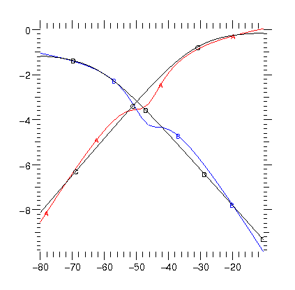
25 July - Porting models The choice not to support arbitrary expressions for state transition rates means that to re-implement existing models requires fitting a Boltzmann type transition to the legacy models. The image shows the type of problem that can arise. In black are the forward and reverse transition rates as a function of membrane potential (log rate in ms against mV). In red and blue are the best fits to these rates. It remains to be seen if there are any functional differences in the behavior of the model.
12 July - Efficient calculation of HH Models So far, HH models (multiple independent two-state gating complexes) have been computed either as the single equivalent scheme, or as a collection of serial two-state gates. This is a little inefficient in the continuous regime, since normally several gates have the same kinetics. This is now exploited in the usual way with an "instances" attribute on a complex to give the power of the gating variable. In the stochastic regime it makes no difference since it is necessary to follow each complex (or the single equivalent complex) in detail in any case.
4 July - Noise and Conductance inputs TBD
6 June 2007 - Stochastic simulation and random numbers. How many random numbers should it take to advance a population of n channels? It can certainly be done with n random numbers. If, as is often the case, for a given start state there is an overridingly popular destination state (probability p), then you only need to use a few times n(1-p) random numbers - just those channels that have a chance of not being in the default destination (often, but not always, the current state). But for some cases it should still be lower than this: eg, first generate the number that change at all, then the number that aren't in the second most popular destination, then you may well have none left at all. But the above two steps could cost more than quite a lot of random numbers, so when is it worth it?
28 May 2007 - KS Scheme equivalents of HH Channels. Hodgkin-Huxley style models - multiple serial independent two state complexes, frequently with several sharing the same properties - are a simple extension of single-complex schemes for the continuous case, but not in the stochastic case. For the former, the complexes can be treated independently, just multiplying up the relative conductances at the end. But for a population of stochastic channels it is not enough to know how many of each type of complex are in each state: you need to know which complex of one type goes with which complex of the other type. So the slow stochastic algorithm is fine, where the state of every complex is recorded, but population based methods do not work.
The current solution is to automatically construct the minimal equivalent single scheme specification from a HH-type model. As yet the procedure is specific to models of type a bn (one type a complex, n type b complexes) but that should cover all interesting cases: for more sophisticated multi-complex models it is probably worth constructing a single-complex equivalent by hand.
Predictable, the performance of single-scheme equivalents is not as good in the continuous regime as the multi-complex version (one 8x8 matrix by vector multiplication costs more than two or even four 2*2 matrix by vector multiplications), so the multi-complex option has been left in for continuous calculations.
May 2007 - Fortran core. Now running, and producing the same results as the Java reference at something between 15 and 50 times faster (though the comparison is not just on the language since they use different methods). The main observation, performance-wise, is that the elegant new (well, newish) features of Fortran 95 are not much use in inner loops: data parallel statements and pointer arrays are substantially slower (using a single core) than their old fashioned equivalents both with GFortran and Absoft. Presumably this is from all the additional copying where "A = A + b" leads to a copy of A being incremented and assigned back to A, instead of the element-wise increment in a do loop. Likewise "forall" is much more costly in the PSICS inner loops than explicit "do" loops. Rather disappointing really, since the data parallel versions are much more readable! And if only Fortran would introduce a "+=" construct to avoid writing complicated index lists twice ("pop%gcs(igc)%states_stoch(p, icpt) = pop%gcs(igc)%states_stoch(p,icpt) + 1" is just something you shouldn't have to write). Pointers would solve the problem, but at the cost of setting the target attribute on the arrays used in inner loops which is probably not smart. On the other hand, automatic allocation (calling a subroutine and declaring that new arrays should be available inside it with sizes that depend in its arguments) is pretty nice.
30 April 07 - Multiple runs and parameter access. The RunSet block now has access to the whole model and allows embedded CommandConfig blocks to do two-dimensional parameter variation. The default behavior is to process a family of commands, such as a sequence of voltage steps, through a single model. Steps are specified in the same way as the RunSet itself by identifying the parameter to vary and setting the values it should take in successive cases. For the RunSet, the target parameter can now be anywhere in the model. It is sufficient to set the id on the component containing the parameter and then to target it from the RunSet with a target of the form id:field where id is the id of the target component and field is the name of the quantity to be varied. This is mainly implemented in ModelMap.java, which could easily be extended to provide unix directory style access to the model - if a need arises.
26 Aripl 2007 - JNI and Fortran There is now an embryonic version of FPSICS (Fortran PSICS) that provides an entry point form Java and has access to a fortran-style serialization of the pre-processed task specification. The outer-core generates the internal structures ready to start the calculation (discretizes the cell, tabulates channel transition rates etc) and writes them to a text file in a "sequentially readable" style - that is, such that a line-based reader can reinstantiate the whole lot without stacking or backtracking (which has a lot going for it in fact). No lines mixing doubles and ints, dimensions declared in advance rather than deduced from the context etc. The latter could be fragile for manual editing, but these things shouldn't be edited by hand.
On an implementation level, Photran with CDT (the Fortran and C development systems for Eclipse respectively) does the trick nicely for calling Fortran from Java. The process is to declare the native method in Java, generate a c header file, write a c wrapper function that calls fortran, write the fortran and then join them together, putting in the name-mangling and string mappings that are needed between the two until there are no linkage errors. With a bit of configuration, the Fortran build can also compile the c and make a shared library with the c as entry point, which is all that java needs. Not much fun, but once it works that should be it.
16 April 07 - Numerical Methods. There is now a "method" attribute to the main run configuration that can take the values "implicit_euler", "crank_nicolson", "weighted_crank_nicolson" (the default) and "forward_euler". These only vary in the values of the temporal difference weighting factor (1.0, 0.5, 0.51, and 0.0 respectively). This factor can also be set explicitly with the tdWeighting attribute, which is mainly intended for exploring the dependence of the results on the numerical method, rather than for normal modeling applications. However, it may also allow better accuracy with large timesteps for quick approximate calculations without the normal Crank Nicolson oscillations by picking values in the range 0.5 to 1.
11 April 07 - Validation site The results of rallpack calculations and any other models in the validation source tree are now published to validation.psics.org. The SiteBuilder class in org.psics.validation regenerates all the html.
April 07 - Rallpack Creating equivalents of the rallpack models required a couple of extensions to the preprocessing step. The first is completion of the implementation of the "minor" flag for points in the structure. This can now be applied to any point and specifies that the segment from its parent is a cylinder of constant radius, rather than tapered as is the default. The discretization also pays attention to minor segments and treats them as the beginning of a new compartment rather than splitting the parent compartment some distance along the segment as it would for a tapered segment. This allows the branching "tin-can" structure of Rallpack 2 to be implemented by declaring all the points in the structure except the first, to be minor.
The Other extension was to add two more possible transition types to cover the expressions used in Rallpack 3 for the HH equations. These are the Exponential, A exp ((V - V0) / B) and Sigmoid, A / (1 + exp ((V - V0) / B) transitions.
March 30 07 - Mesh generation 2 The comments below (February 07) turn out to be misguided. The "remeshing problem" is only a problem if you require compartments to be straight cylinders. But there is no reason why they should be. Removing this constraint and returning to the numerical objectives yields a simple solution. Just use the structure exactly as it is and discretizes into subsections according to the needs of the numerical method and accuracy constraints (just as one would for any other pde problem...). The result is that you get compartments with bends or even branches in them, so there is a slight increase in computational bookkeeping to compute areas and axial resistances, and a bit more work to draw them. But these are all straightforward processes and implementing them has the double benefits of not changing the structure for the convenience of the calculation, and not tying the hands of the calculation by the details of the structure.
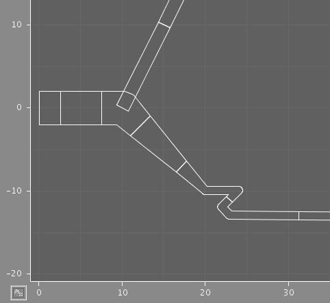
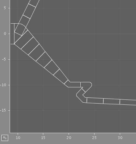
The two images illustrate the results of using different discretization criteria on a section of dendrite. In each case, some compartments comprise multiple points from the original structure, but the shape is preserved.
March 07 - Java inner core First complete runs using channel models and extended cells. The stochastic calculation is only channel-by-channel, but gives quantitative agreement with the ensemble method. Channel distribution is handled with an external expression parser - jep - which is wrapped in an Evaluator class so alternatives can be easily switched in if necessary (a graph reduction parser might be easier to modify for mixing extra morphology conditions in with the expression). Output is currently only ad-hoc text for viewing with CCViz
2 February 07 - Mesh generation Probably the trickiest part of preprocessing morphologies is the compartmentalization since it presents a number of potentially incompatible requirements. Between two successive branch points one would like to change then number of segments, but preserve: end point positions; total surface area; total volume; axial resistance; radius profile with path-length; position profile. In general they can't all be satisfied (except for refining-only discretizations). The simplest case is for a wiggly section of dendrite that should be approximated by a few longer segments. Just evening out the wiggles will give too low a total length, capacitance, etc. The optimum for most criteria is likely to be a zig-zag between the end points.
The current strategy has two steps:
- decide on the number of segments and interpolate between the two branch points to position them on the profile.
- iterative refinement to adjust point positions and optimize some function of the possible metrics to achieve the best fit under given criteria.
28 January 07 - Neuron Imports Two new packages, org.psics.models.neuron and ...neuron.lc (Lower Case) for importing morphologies from neuron. They contain mostly small java classes that are instantiated by reflection on reading a neuron file. The "getFinal" methods generate standard PSICS morphologies, enabling the formats to be read without any specific handling code other than to recognize which packages should be searched when parsing these formats.
January 07 Format specifications and website.